
An evolutionary algorithm (EA) is applied to a given problem task for a fixed amount of clock time. The state of the EA is then read (sampled), and the EA is reset and run again with a different random seed. This process is repeated a large number of times resulting in a set of samples from which histograms can be constructed.
Most notably a histogram of the best fitness achieved in each EA invocation captures and describes the efficacy of an EA on a given task, i.e. the range of best fitness scores achieved and their relative frequency when the EA is run multiple times.
When applied to the same task different EAs will result in different histograms, thus efficacy sampling provides a means of comparing efficacy of different EAs (or variants of an EA) on the same task. In particular, if some change to an EA were to effect its operation in any significant way then the shape of the histogram it produces will change, even though various simple statistics may not necessarily change, such as median or mean best fitness. That is, a histogram gives a richer description of the efficacy of an EA on a task than simple statistics or moments.
The definitive measure of an EA's efficacy is the speed at which it can find solutions for a given amount of computing resource. I.e. the ultimate goal of any search algorithm is to find what is being sought as quickly as possible on a given computing hardware platform. As such the term efficacy is used in this paper to refer to the overall performance of an evolutionary algorithm, resulting from a combination of the innate or direct efficacy of the algorithm (does it work) and its speed of execution, e.g. does the software make good use of available hardware acceleration.
E.g. efficacy sampling provides a means of comparing an EA that finds good solutions but that executes very slowly, with a poor EA that executes very quickly, such that overall the two algorithms may give similar results in a given amount of clock time.
It is necessary to take this combined efficacy and speed approach because the overall efficacy of an EA is typically dependent on indirect or second order dynamics, such as the interaction between a mutation rate and a crossover rate, or different types of mutation, or any number of other EA parameter variations and combinations thereof. E.g. if a crossover rate is increased then the crossover execution path will be executed more often, and therefore the speed of that code path becomes more relevant to the efficacy of the EA as a whole.
Or, a certain type of mutation may influence the size and complexity of the evolved solutions. In turn the speed of the decode phase (if one is required) and phenotype code execution (e.g. a neural network implementation) becomes more or less relevant in an overall efficacy measure if the genome size is larger or smaller on average.
Furthermore, certain algorithms may inherently run faster on certain types of CPU (e.g. AMD versus Intel CPUs), perhaps because some CPU has more floating point units and the computation is floating point maths heavy; or maybe some EA has specific optimizations using SIMD vector instructions, or GPU resources, etc.
The resulting complex set of interactions and dynamics can be measured effectively by a high level efficacy measure as defined in this paper. Performance of individual subroutines still matters, but the degree to which they matter varies in complex ways depending on many different factors.
A histogram can be constructed for a continuous variable by dividing the continuous range of the variable into multiple contiguous discrete sub-ranges (or 'bins') and counting samples into those bins, thus describing the relative frequency of samples in each bin. In this mode a histogram is essentially an approximation of some underlying true continuous distribution; an approximation that approaches the true distribution as the sample count approaches infinity and the bin range approaches zero (i.e. with narrowing bin range).
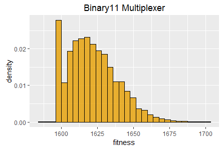
The efficacy of an EA on a given task has such a continuous underlying distribution that is essentially sampled by construction of a histogram. Of note is that the histograms produced by efficacy sampling often contain a large proportion of samples within a very narrow range or at a single value. This occurs because some proportion of the EA invocations can become 'stuck' at the same fitness level. Hence a histogram may essentially be representing both a discrete distribution (the number of samples from some single special case scenario), and a continuous distribution.
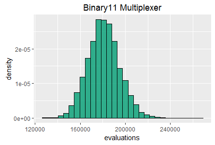
In the true underlying continuous distribution the special case occurs as a distinct spike, whereas in a histogram the samples in the spike fall within the range of one of the bins and are therefore 'averaged down', manifesting as a slightly higher frequency in one of the bins rather than as a distinct spike. Such an effect can be observed in the binary11 multiplexer histogram in figure 1. This effect can be mitigated somewhat by taking more samples and reducing the bin range.
As described above, the efficacy measure defined in this paper incorporates the execution speed of an EA, which in turn is dependent on the computing hardware on which the algorithm runs and whether the software has any particular optimizations when running on that hardware. As such, in order to make direct comparisons between different EAs they must be executed on the same computing hardware, and ideally they would all make use of any acceleration primitives (e.g. SIMD instructions) available on that hardware.
If some EA does not make use of available acceleration primitives then it is at an immediate disadvantage relative to EAs that do. Ideally we would seek to eliminate these differences such that we are comparing high level algorithms and not implementation details. Ultimately however if some EA implementation provides significant optimizations and another doesn't, then the efficacy measure will favour the faster code; this is intentional and by design, i.e. the efficacy measure reflects real world performance, not hypothetical performance should additional performance optimizations be made.
An evolutionary algorithm will typically have a number of parameters such as population size and mutation and crossover rates.
When comparing two or more EA implementations it is necessary to choose a set of parameters for each EA that are considered good choices (or in fact the best choice possible) for each of those EAs, independently of the choices made for the other EAs. That is, each implementation should be configured using the best knowledge available regarding how to achieve the best results for that EA. Specifically, it is not necessary to match parameters, e.g. if two EAs both have a mutation rate then it is not necessary to configure the rates to be equal when comparing those EAs.
Two stopping conditions have been chosen as being particularly useful. (1) The passage of a fixed amount of clock time; (2) The execution of a fixed number of generations. Note however that not all EAs are 'generational' in nature, hence (2) may not be possible for all EAs.
These two modes of sampling measure different aspects of efficacy. A clock time stopping condition gives the definitive measure of efficacy. However, using the generation count stopping condition may be useful for comparing results from a single EA implementation running on different hardware, such that the speed of the hardware is factored out of the efficacy measure. Note however that such a comparison is valid only for the exact same EA implementation (with the exact same parameters), otherwise a parameter change may cause the EA to perform a qualitatively different search which may lead to the number of generations having a poor correlation with actual resource usage (e.g. consider the increased resource usage when genomes rapidly become very large, versus staying relatively small).
Two standard tasks were chosen for efficacy sampling experiments in this paper; (1) Binary11 Multiplexer; (2) Generative Sinewave.
Eleven binary inputs are defined as three 'selector' inputs that between them can take one of eight binary values; and eight 'signal' inputs. A single binary output is required to take the value of the signal input that is selected for by the three selector inputs. Evaluation is performed by enumerating all 211 (=2048) possible input combinations and testing for the correct response at the single output.
Binary11 Multiplexer is a highly non-linear task and as such is challenging for neural network based EAs. It is however very fast to execute, hence computing resource can be largely devoted to executing the evolutionary search algorithm rather than task specific code.
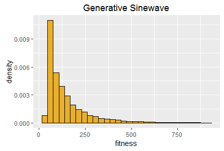
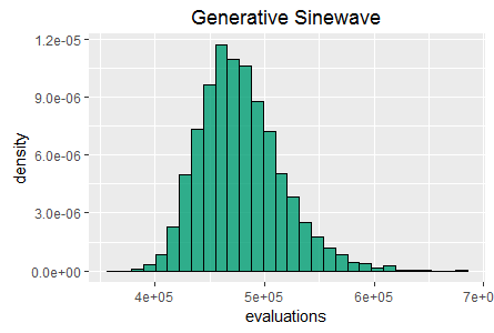
In this task there are no inputs and a single continuous output that is required to generate a sinewave in the time dimension. This task therefore requires phenomes to have internal state that they can update, and is therefore suitable for testing the evolution of cyclic/recurrent neural networks. This task is also very fast to evaluate, requiring trivial amounts of CPU and RAM.
SharpNEAT (version 2.2.4) was applied to the two standard tasks defined above. The specific search parameters and hardware platform details are listed below (appendix 1). A stopping condition of 60 seconds of clock time was used, and EA statistics read at the end of those 60 seconds. Histograms of best fitness are shown in figure 1 (above).
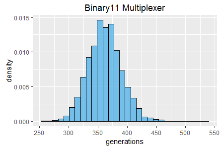
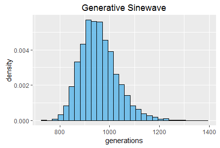
Further histograms of generation count and total evaluation count (also at 60 seconds) are shown in figures 2 and 3.
NEAT employs crossover recombination as a key part of its evolutionary search strategy. SharpNEAT has a long standing default crossover rate setting of 50%, i.e. 50% of offspring (new genomes) in each generation are produced by application of crossover recombination applied to two randomly selected parent genomes. The remaining 50% of genomes are produced by mutation of randomly chosen single parent genomes.
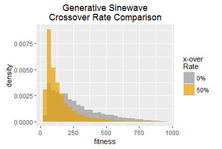
In this experiment SharpNEAT is applied to the same two tasks as in experiment 1, with all of the same parameters except for the crossover rate which is set to 0%; i.e. all new genomes are produced by genome mutation only. The resulting histograms of best fitness are show in figure 4 overlaid with the histograms from experiment 1.
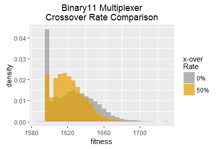
Note that both tasks result in qualitatively distinct histograms for the two crossover rates. The Binary11 Multiplexer task appears to become stuck at a low fitness score approximately twice as frequently when crossover is disabled. However, some of the highest scores in the histogram also occur more frequently (with crossover is disabled).
In the Generative Sinewave task it is the 50% crossover rate that appears to result in fitness becoming 'stuck' at lower scores approximately twice as frequently. However, once again disabling crossover results in higher frequencies for some of the highest scores. Interestingly the very highest scores in both tasks are achieved by the 50% crossover rate, thus these experiments suggest that crossover results in a complex mix of benefits and disadvantages, rather than clearly being beneficial or disadvantageous overall.
The primary motivation for the development of efficacy sampling is the ongoing development of SharpNEAT; in particular as a means of evaluating proposed modifications and enhancements, but also as a high level test when making more significant changes to the software. That is, efficacy sampling can be used to ensure that a newer code base continues to work at least as well as previous versions of the software, and that no inadvertent subtle defects have been introduced.
However, it is hoped that the general approach may be useful to the wider evolutionary search research community.
Experiments 1 and 2 were run using SharpNEAT's default parameters, except for experiment 2 in which the crossover rate was set to 0%. The full set of parameters and all of the source code used for these experiment is available on github ( SharpNEAT version 2.3.4). However, the key high level parameters are listed below.
| Setting | Value | Notes |
|---|---|---|
| Population Size | 600 | |
| Species Count | 40 | |
| CPU Cores | 4 | Max number of CPU cores to utilise. |
| Crossover Rate | 50% | Proportion of new offspring to produce from crossover. |
| Interspecies Crossover | 1% | Proportion of crossovers between parent of different species. |
| Elitism Proportion | 20% | The proportion of the population (ranked by fitness) to maintain between generations (the remainder of genomes are discarded and replaced with new offspring). |
| Selection Proportion | 20% | The proportion of the population (ranked by fitness) to select for creation of offspring genomes. |
| Weight Mutation | 94% | The proportion of mutations that are weight mutations. |
| Add Node Mutation | 1% | The proportion of mutations that are 'add node' mutations. |
| Add Connection Mutation | 1% | The proportion of mutations that are 'add connection' mutations. |
| Delete Connection Mutation | 1% | The proportion of mutations that are 'delete connection' mutations. |
OS Name: Microsoft Windows 10 Home SP0.0
Architecture: 64-bit
FrameworkVersion: 4.0.30319.42000

CPU 0
   Brand: GenuineIntel
   Name: Intel Core i7-6700T CPU @ 2.80GHz
   Architecture: x64
   Cores: 4
   Frequency: 2808
   RAM: 16 GB
Colin,
April 2nd, 2017
 Copyright 2017 Colin Green.