Equations of Motion for the Cart and Pole Control Task

Colin D. Green

1. Introduction

The cart and pole task is a classical benchmark problem in control theory and reinforcement learning [3,2,4], also known as the inverted pendulum, or pole/stick/broom balancing task. This paper provides derivations for the equations of motion for the cart and pole task, and accompanying discussions and analyses.

From Lunberg and Barton [3]:

The inverted-pendulum system is a favourite example system and lecture demonstration of students and educators in physics, dynamics, and control. This system is a simple and valuable laboratory representation of an unstable mechanical system. It is also often used to model the control problems encountered in the flight of rockets and missiles in the initial stages of launch, when the airspeed is too small for aerodynamic stability.

Section 2 of this paper defines the cart and pole physical model. In section 3 we derive the equations of motion for the model, for a single pole and also for multiple poles. Section 4 discusses a hybrid model that is ubiquitous in the literature, and presents adapted equations for that hybrid model.

Appendices C, D and E provide analyses of the cart and pole equations presented in three well cited sources from the literature, highlighting errors, and discussing variations in the published equations.

Finally, appendices A and B provide a brief overview of d'Alembert's Principle and Torque, respectively, in support of the derivations in section 3.

1.1 Terminology: Pendulums, Poles, and Sticks

For conciseness we will generally refer to the cart-pole task, model, or system, rather than the 'cart and pole balancing task' or 'inverted pendulum balancing task', etc., and pole is generally preferred over inverted pendulum or stick.

The word pendulum may occasionally be used when discussing oscillation or rotation of the pole around its pivot point, thus emphasising that the pole is behaving as a pendulum. Furthermore, pendulum will generally refer to an ideal pendulum unless otherwise stated, i.e. a point mass attached the end of a massless rod.

2. The Cart-Pole Physical Model

Consider the physical model shown in figure 1. A cart is positioned on a track running horizontally, and an inverted pendulum is attached to the cart with a hinge that allows rotation around pivot point P in the xy plane only, i.e. the pendulum is free to fall horizontally left-right, but not 'out' of the diagram. The pendulum's initial position is near vertical, and a external variable horizontal force is applied to the cart to maintain the pendulum in a balanced and upright position.

The model is considered to represent an unstable system because an external control force is required to keep the pendulum balanced; as opposed to a downward hanging pendulum in which the force of gravity alone results in stable oscillation about the downward vertical.

We will assume an ideal pendulum, in which all of the pendulum's mass is located at a single point (Q) at the end of a massless rigid rod.

Table 1: Symbols used in figure 1 and throughout this paper

$x, y, O$	A Cartesian x, y coordinate frame is shown, with origin O.
$C$	The cart's centre of mass.
$P$	Pivot point of the inverted pendulum.
$Q$	The pendulum's point mass. At distance $l$ from point P.
$l$	Length of the pendulum rod.
$T,R$	An alternative coordinate frame with the R axis parallel to the pendulum (vector PQ). I.e. the TR coordinate frame rotates and moves horizontally relative to the fixed (or 'world') Cartesian coordinate frame.
$x$ (lower)	Horizontal position of the cart on the track.
$\theta$	Angle of the pendulum in radians, measured as a deviation from the vertical. The pendulum is at 0° when oriented vertically straight up, +90° when horizontal and to the right of the pivot point, -90° when horizontal and to the left of the pivot point, and +-180° when oriented vertically down.
$m$	Mass of pendulum's point mass at point Q.
$g$	Gravitational acceleration (in m/s2). Here g is taken to be the directionless magnitude of the acceleration caused by gravity (i.e. approximately 9.8 m/s2 for gravity on Earth). The direction of gravitational acceleration is taken into account in the formulation of the equations, therefore the sign of g is positive.
$f$	An external variable horizontal force applied to the cart (in Newtons). A positive value represents a push to the right, and a negative value represents a push to the left.

Selected additional symbols used throughout this paper:

$\dot x, \ddot x$	The cart's x-axis velocity and acceleration, respectively.
$\dot x_q, \ddot x_q$	Point Q's x-axis velocity and acceleration, respectively.
$m_c$	Mass of the cart.
$M$	Combined mass of the cart and the pendulum, i.e. $m_c + m$
$\hat l$	Half length of the pendulum rod.

Conventions:

A positive horizontal force represents a push to the right.

A positive vertical force represents a push upwards.

A positive angular velocity represents clockwise rotation.

A positive angular acceleration represents clockwise acceleration.

A positive moment (also know as torque or a rotational force) is a rotational force in the anticlockwise direction (see appendix B for an explanation). I.e. a positive torque results in negative angular acceleration.

3. Equations of Motion (Derivations)

3.1 Acceleration of point Q relative to point P

The position of Q relative to P in the XY coordinate frame, and for a given pendulum angle $\theta$, is given by:

Taking the derivative of (1) and (2) with respect to time gives the XY velocity of Q relative to P, for a given pendulum angle $\theta$ and angular velocity $\dot\theta$.

Velocity (x-axis):

Velocity (y-axis):

Taking the derivative of (3) and (4) w.r.t. time gives the XY acceleration of Q relative to P, for a given pendulum angle $\theta$, angular velocity $\dot\theta$ and angular acceleration $\ddot\theta$.

Acceleration (x-axis):

Acceleration (y-axis):

The above equations describe the XY motion of point Q given it's motion stated in polar coordinate system terms of angle and distance from the pivot point. These equations say nothing about the forces acting on the system that are the cause of the motion.

Equations (5) and (6) show that there are two distinct effects that contribute to the acceleration of Q relative to P, manifesting as two separate terms in each equation; a term dependent on rotational velocity ($\dot\theta$), and a term dependent on rotational acceleration ($\ddot\theta$).

The terms dependent on velocity describe the centripetal acceleration acting on Q, continuously pulling Q directly towards the centre of rotation (point P) and thus maintaining circular motion. Noting that the centripetal force $F_c$ for a mass $m$ at a given radius $r$ and angular velocity $\omega$ is given by:

$$ F_c = mr\omega^2 $$

We can perform a basic check of equation (5) by confirming that the x-axis component of the centripetal term is zero when the pole is vertical, and at its maximum when the pole is horizontal. And similarly for equation (6), the y-axis component of the centripetal term is zero when the pole is horizontal, and at its maximum when the pole is vertical.

The other component of equations (5) and (6) is dependent on angular acceleration ($\ddot\theta$). This gives the x and y-axis accelerations of Q for a given angular acceleration and point Q's distance from the centre of rotation (P). A simple check here is to confirm that this acceleration is always perpendicular to the pendulum (line PQ), as opposed to the centripetal acceleration that is always parallel to PQ. These angular acceleration components are essentially describing the relationship between rotational force on the pendulum, i.e. torque, and the resulting force on point Q.

3.2 Absolute Acceleration of Point Q

Equations (5) and (6) describe the acceleration of point Q relative to P. Therefore to obtain the absolute acceleration of Q (i.e. acceleration relative to point O, or the 'world' XY frame) we add the x-axis acceleration of point P to equation (5). The cart does not move vertically, therefore the absolute y-axis acceleration is given by $\ddot y_{q|p}$.

Absolute acceleration (x-axis):

Absolute acceleration (y-axis):

In Cannon [2] a vector notation is used as well as an alternative coordinate frame TR (shown in figure 1), use of which results in the following more concise definition of Q's acceleration:

$$ \mathbf{a}^Q = \mathbf{1}_x(\ddot x) + \mathbf{1}_T(l\ddot\theta) + \mathbf{1}_R(-l \dot\theta^2) \tag{9} \\[2ex]$$

Where $\mathbf{1}_x()$ denotes a unit vector in the x-axis, $\mathbf{1}_T()$ denotes a unit vector in the T-axis of the RT coordinate frame, and so on.

3.3 Inertial Force on Point Q

We now adopt d'Alembert's principle (see appendix A).

The pendulum's mass at point Q resists acceleration, resulting in an inertial force (denoted with a superscript i) with a direction opposite to the direction of acceleration. We obtain this force by multiplying equations (7) and (8) with the pendulum's mass (m) as per Newton's Second Law of motion $F=ma$, and changing the sign to obtain a force in the opposite direction to the acceleration of Q:

Inertial force (x-axis)

Inertial force (y-axis)

3.4 Forces on the Cart

The external forces on the cart are the external horizontal force f, and a force transmitted by the pendulum rod at point P resulting from the inertial resistance of the pendulum mass at point Q, and also gravity acting on that same mass. In addition there is the cart's own inertial resistance, i.e. the cart's resistance to acceleration.

Given that the cart does not move vertically, it is sufficient to constrain our analysis here to the horizontal forces acting on the cart; these are force f, the horizontal component of the pendulum's inertial force (given by equation 10), and the cart's inertial force. Summing these forces and and equating to zero as per d'Alembert's principle, we obtain:

Equation (12) matches the first equation of (22.55) in Cannon [2]. This indicates that Cannon used the convention of a positive force being a push to the right for the cart-pole equations, whereas the opposite convention is used elsewhere in that book. I.e. Cannon states (§2.2 pg40) "...it is convenient to choose to make the positive direction for each force opposite to that for the corresponding motion, and we shall normally do so in this book, purely for convenience."

To demonstrate the point, note that the $m_c \ddot x$ term represents the inertial force resulting from acceleration of the cart; this force is in the opposite direction to the cart's acceleration, thus we see that a positive acceleration results in a negative inertial force in the two equilibrium equations leading to equation (12).

3.5 Rotational Forces on the Pendulum

We now turn our attention to the rotational forces acting on the pendulum. A rotational force is referred to as a moment, moment of force, or torque

There are three forces that result in a torque acting on the pendulum, these are (i) gravity acting on the pendulum's point mass at Q; (ii) the inertial force resulting from the inertial resistance of the pendulum's point mass at Q, i.e. as the cart moves left or right beneath the pendulum; and (iii) a rotational inertia force known as the moment of inertia. The three resulting torques must be in equilibrium as per d'Alembert's principle, giving an additional equation of motion for the cart and pole model.

The inertial force on Q is given by $F^i_q$, as defined in equations (10) and (11). Taking the cross product of vectors $\mathbf{1}_R(l)$ (i.e. radial vector PQ) and $F^i_q$ gives a vector that points along the axis of rotation, with the magnitude and sign of that result vector giving the magnitude and sign of the torque at pivot point P resulting from force $F^i_q$ (see appendix B for an explanation and a brief introduction to torque). Given that we know that the axis of rotation is fixed and is parallel with the z-axis, the result vector's magnitude and sign is given by its z-axis component alone, as follows:

$\mathbf{M}_q$ is the moment of inertia resulting from the point mass at Q.

The cross product operation is not commutative, therefore it is important that the operands in equation (13) are in the correct order; this is determined by the right hand rule. The direction of cross product $a \times b$ can be determined by imagining vector $a$ turning towards vector $b$ (in the direction of the the smallest angle between those two vectors). If turning $a$ towards $b$ results in a right handed screw advancing into the plane of rotation, then this is clockwise rotation, and in our model the result vector has a negative z-axis component (see Table 1 - Conventions).

Thus, if we imagine a positive force $F^i_q$ pushing an upright pendulum to the right then we would expect this to cause clockwise rotation, and therefore negative torque (see Table 1 - Conventions).

Equation (13) appears as a term in Cannon [2] equation (22.53), and again in the fourth equation of (22.54). The minus signs in those two equations (from Cannon) are inconsistent and erroneous. Specifically, the moment in (22.53) should not be preceded by a minus sign, rather, the torque force (with whatever sign it happens to have) should be summed wth the other moments to form the equilibrium equation. However, the error in (22.53) is cancelled out by another sign error in the last equation (22.54); in that equation the left hand side is prefixed with a minus sign, but the right hand side gives the cross product that results when that minus sign is not applied.

The torque resulting from the downward pull of gravity on the pendulum's mass at Q is given by:

Noting that the torque resulting from gravity is zero when the pendulum is fully vertical, and negative when the pendulum is at +90°, i.e. accelerating the pendulum with a negative torque, and therefore in the clockwise direction.

In Cannon [2] the moment of inertia is initially written as some multiple (J) of $\ddot\theta$, to be substituted later; we will do the same here:

Noting that the sign of $M_i$ is positive for positive $\ddot\theta$, representing a positive and thus anticlockwise torque when the pendulum is accelerating clockwise.

Summing the three moments and equating to zero as per d'Alembert's principle, gives:

Equation (18) matches the second equation of (22.55) in [2].

3.6 Combining Horizontal and Rotational Force Equations

Equation (12) describes the horizontal forces acting on the cart in equilibrium; and equation (18) describes the moments (rotational forces) acting on the pole in equilibrium. These two equations can be combined and rearranged to arrive at a complete set of equations for the cart-pole model.

Firstly, it is useful to rearrange equations (12) and (18) to give the accelerations $\ddot x $ and $\ddot\theta$ for a given external force $f$.

Rearranging (12) to give $\ddot x$:

Rearranging (18) to give $\ddot x$:

Equating the right hand sides of (19) and (20), and rearranging to give $\ddot\theta$:

Equation (21) can now be evaluated at each timestep to obtain $\ddot\theta$, and the result substituted into either (19) or (20) to obtain $\ddot x$; thus equations (19), (20) and (21) are sufficient for simulation of the cart-pole physical model, provided that a suitable definition for $J$ is substituted in.

We can also arrange (12) and (18) such that we evaluate $\ddot x$ first, and substitute its value into an equation for $\ddot\theta$, i.e. a new set of equations that are alternatives to equations (19), (20) and (21):

Rearranging (12) to give $\ddot \theta$:

Rearranging (18) to give $\ddot \theta$:

Equating the right hand sides of (22) and (23), and rearranging to give $\ddot x$:

Note. Equations (20) and (22) have an undefined result when $\cos\theta$ is zero, therefore these equations should be avoided for obtaining $\ddot x$ and $\ddot\theta$. Equations (19) and (23) serve the same purpose and therefore these are preferred.

3.7 Applying a Rotational Inertia Constant

The rotational inertia of a point mass at fixed distance $l$ from the axis of rotation (as per our pendulum), is given by (see List of moments of inertia):

However, the following alternative definition for $J$ is given by Cannon [2]:

This is the moment of inertia for a pole of length $l$ with uniformly distributed mass along its length, and although not stated explicitly elsewhere the use of this definition is ubiquitous in the literature (see appendices C, D and E). The reasoning for this choice is discussed in Appendix C: The Equations of Cannon, but regardless of that reasoning, what we can say is that of the various definitions of $J$ that we may elect to apply for a pendulum, they are all some constant multiple of $ml^2$. As such the above equations may be simplified with the following substitution:

Where $k$ is some constant to be substituted later. Substituting (25) into (21), (23) and (24), and repeating (19) to show the final set of equations together:

(25) into (21):

(25) into (23):

(25) into (24):

These equations present the following three options for finding values for $\ddot x$ and $\ddot\theta$.

1. Equation (26) can be evaluated to obtain a value for $\ddot\theta$, and the result substituted into equation (19) to obtain a value for $\ddot x$.


2. Equation (28) can be evaluated to obtain a value for $\ddot x$, and the result substituted into equation (27) to obtain a value for $\ddot\theta$.


3. Equations (26) and (28) can be evaluated to directly obtain $\ddot\theta$ and $\ddot x$, respectively.

Options 1 and 2 are generally preferred as they avoid redundant recalculation of intermediate results.

3.8 Friction

The most significant sources of friction in the cart-pole system are (i) friction between the cart and the track, (ii) friction in the pendulum's pivot joint, and (iii) air resistance. The equations given in the literature generally model the first two types of friction, or no friction at all; here we will examine the first two types, omitting air friction.

Friction is necessarily modelled with an approximation as it is the result of many complex processes at many scales, such as atomic forces, microscopic and macroscopic structure, and factors such as vibration, dirt and dust ingress between moving surfaces, fluid dynamics (if lubrication is used), etc.

For sliding/translational friction between two flat surfaces we employ the Coulomb approximate model of friction. This model defines a friction force given by the product of (i) the force pressing the two surfaces together (know as the normal force), and (ii) the coefficient of friction between the two surfaces (with a rough surface having a higher coefficient of friction than a smooth surface). Notably, Coulomb friction is not proportional to contact surface area or velocity of the sliding object.

For rotational friction (also know as torsional friction) Cannon [2] suggests a model (§2.2, figure 2.4e, pg 42) that defines a friction force that is proportional to angular velocity; this is consistent with a lubricated ball bearing joint in which the lubricant surrounding the bearings reduces friction greatly, but also introduces fluid friction caused by viscosity of the lubricant. The friction in such a bearing is typically very low (e.g. compared to sliding dry friction) therefore although the friction increases with angular velocity, the coefficient of friction will typically be so low as to result in only a small friction force, especially at the relatively low angular velocities expected in the cart-pole system.

Regarding static friction, we have chosen not to model this. For one, the cart-pole system could be considered to be in constant motion, or we could claim that static friction is minimal in the wheels and the pole pivot joint. From a practical point of view an exact zero velocity will occur (i) when the cart-pole system begins from a stationary state, and (ii) when the cart and pole change direction of motion as they oscillate back and forth during balancing. Scenario (i) exists only for a single initial instant and therefore doesn't affect the overall dynamics of the system thereafter.

Scenario (ii) is more problematic, it will hardly ever (or never) be observed precisely upon a simulation timestep (see §6 Numerical Integration), rather, it will occur between timesteps, resulting in an instantaneous and discontinuous change in the forces acting on the system partway between two consecutive timesteps. As such, the proper handling of static friction (occurring as the result of instantaneous zero velocities) requires additional complexity around the detection and handling of the zero velocity states, in exchange for what is likely a minimal improvement in modelling quality. Hence the choice to not model static friction is in keeping with Cannon's guidance regarding judgement of which real world physical characteristics to model and which to omit (see appendix C for further discussion on this point).

Finally, note that friction is always a force that acts in the opposite direction to the direction of motion, i.e. friction is always a retarding force on motion; we can use this fact to make basic sign checks on the friction force terms.

Figure 1 shows a cart with wheels which would typically contain lubricated low friction wheel bearings as the primary source of friction between the cart and the track. Alternatively we could choose to model the cart as a solid block sliding along a flat surface (with horizontal guides to prevent the cart sliding sideways).

Cart-track sliding friction as defined by Coulomb's law is given by:

Where $N_c$ is the normal force between the cart and the track, and $\mu_c$ is the coefficient of friction between the cart and the track. The normal force consists of two counteracting forces; the downward vertical force being applied by the cart onto the track, and an opposing upwards force being applied by the track onto the cart, preventing it from falling through the ground. The magnitude of these two forces is equal, with the downward force having a negative sign, and the upward force having a positive sign. We take the absolute value of this force and therefore either of the two forces can be used as the value for $N_c$.

Alternatively we could model cart-track friction as originating from rotation of the cart's wheel bearings:

I.e. in this model cart-track friction is proportional to cart velocity. Note that we divide cart velocity by wheel radius $r$ to obtain the wheel angular velocity, and that the coefficient of friction in this model will tend to be much lower than for sliding friction.

Here we treat $N_c$ as a scalar that represents the magnitude and sign of the vertical normal force. As an alternative we could have treated it as a vector. Either way, $|N_c|$ gives the magnitude of the normal force between the cart and the track, i.e. the vertical bar notation defines the absolute value of a scalar, and the length of a vector (also known as the modulus or magnitude of the vector).

In principle a pendulum with a very high rotational velocity and/or a high mass could result in enough centripetal force to overcome gravity and therefore pull the cart upwards and off the track. In that scenario the normal force applied by the cart onto the track changes to a positive sign (upwards force) and our friction equations become invalid. To address this we could say that we expect the system to never approach such a state, or we could say that a special kind of cart-track system is in use that prevents the cart from derailing, e.g. roller coasters use up-stop wheels to prevent the car from derailing. When the up-stop wheels are applying a force they will also produce friction, and if we assume that their co-efficient of friction is the same as for the normal wheels then equation (29) remains valid.

This may seem to be an unnecessary discussion about a model state that is generally not of interest, but it's important to be aware of such details. A computer simulation could experience such states unexpectedly, and if they aren't properly considered then the fact that such a state occurred and potentially invalidated the whole model may go unnoticed.

The vertical/normal force applied by the cart onto the track is the result of the combined weight of the cart and pole (i.e. the gravitational pull on the cart and pole), and a varying force resulting from motion of the pole.

Note the sign of the force resulting from the pendulum mass at $Q$ resisting the centripetal pull towards pivot point $P$ (given by the $\dot\theta^2$ term); this is a positive (upwards) force when the pendulum rod is upright, i.e. the pendulum mass pulls the cart up as expected.

Substituting (30) into (29):

Alternatively, if the pendulum mass is low and/or its angular velocity is always low, then a reasonable approximation of (31) can be obtained by dropping the component of the normal force resulting from motion of the pendulum, giving:

Noting that if the pendulum is being successfully balanced, its angle will tend to vary only slightly and with moderate angular velocity, i.e. this approximate normal force will only deviate significantly from the true force if the pendulum is swinging wildly. If the pendulum does happen to swing with high angular velocity then perhaps a more appropriate normal force approximation is based on the weight of the cart only, not including the pole.

I.e. in general some constant magnitude with a sign opposite to the cart's direction of motion is a reasonable approximation for the cart-track friction force.

However, a constant friction force based on the sign of the velocity term is not conducive to simulation of the cart-pole system. This is because simulation requires use of a numerical method (see §6) to obtain updates to the model state variables (i.e. the position and velocity of both the cart and the pole) at successive discrete timesteps, and such numerical methods are based on calculating the gradient (i.e. instantaneous rate of change) of each state variable and projecting those gradients forward in time to obtain a new model state one timestep in the future. The use of a constant friction term that changes sign only, results in a discontinuity in the gradients about velocity zero, and this discontinuity greatly impedes the ability of any numerical method to accurately project forward to the correct state at the next timestep.

I.e. e.g. if the velocity zero crossing occurs halfway between two timesteps, then the friction force may be applied in the wrong direction for the latter half of the timestep interval, thus propelling the cart rather than retarding its motion. As such, a friction force that is proportional to velocity is a more practical approximation, as it results in a continuous gradient about zero velocity:

The joint that connects the pole to the cart will also exhibit friction, resulting in an additional moment (rotational force) that retards rotation of the pole. This friction is the result of surface contact within the joint, and as such this rotational friction can also be modelled with Coulomb's Law.

Where $\mathbf{M}_f$ is the moment of friction, $\mu_p$ is the joint's coefficient of friction, and $N_p$ is the normal force between the pole and the cart. Note that a positive (clockwise) angular velocity will result in a positive (anticlockwise) torque/moment (see table 1 - Conventions), hence no minus sign is required.

The normal force in this case is a force with varying direction, i.e. the internal surfaces within the joint that meet under force depend on the angle of the pole and the direction of the force being applied by the pole onto the cart. As such $N_p$ should be considered to be vector. Here we treat the x and y components of that vector separately:

The magnitude of vector $N_p$ is given by Pythagoras' theorem:

As with cart-track friction we may wish to employ a simpler approximation of cart-pole friction by replacing the normal force equation with a constant normal force. In this case the average normal force that is observed depends very much on the dynamics of the system, i.e. e.g. whether the pole remains balanced or swings wildly. As such there is no clear obvious choice for a single constant normal force that is reasonable in all scenarios. In light of this a positive value somewhere in the interval $(0,mg]$ is the next best option, e.g.:

As another alternative Cannon suggests modelling rotational friction as being directly proportional to angular velocity ([2] §2.2, figure 2.4e, pg 42).

As discussed above (§3.8, ¶4), this model is more consistent with a lubricated ball bearing joint, which we may consider to be more appropriate in situations where high angular velocities are expected, perhaps in the hundreds or thousands of rpm range, such as in a motor car engine.

We could also choose to extend equation (40) with a normal force term, as the force being applied through the bearing will affect its behaviour. E.g. perhaps one reasonable choice is:

Where $\tilde\mu_p$ is an additional coefficient of friction that applies to the normal force only. This independent linear scaling may be appropriate for low forces, whereas high forces may cause the bearing to distort, resulting in non-linear changes in friction that also affect the first (angular velocity) term.

Overall we expect the forces through the pole's pivot joint to be minimal and to have a minimal affect on joint friction. Furthermore, the use of a friction force based only on the sign of the angular velocity will result in a discontinuity in the equations of motion (as discussed above in relation to the cart-track friction), therefore we prefer a friction force proportional to velocity as given by equation (40).

As a final alternative, we may consider pivot joint friction to be so low as to be inconsequential, especially if cart-track friction is being modelled, i.e. so long as there is friction somewhere in the model.

The force equilibrium equations (12) and (18) can be extended to include the friction forces $F_f$ and $\mathbf{M}_f$, giving the following equations of motion. These are equations (19), (26), (27) and (28) extended to incorporate friction forces:

Equation (19) extended to include friction:

Equation (26) extended to include friction:

Equation (27) extended to include friction:

Equation (28) extended to include friction:

3.9 Multiple Poles

The task of balancing the inverted pendulum can be made more difficult by attaching a second pendulum to the cart. This new two pole task becomes increasingly difficult as the two pole lengths approach the same length, becoming impossible when they have identical lengths. Extending the task to three or more poles provides a further option for increasing task difficulty in a different way. Here we derive the equations of motion for N poles.

Equation (10) gives the horizontal force applied by a single pole onto the cart; we rewrite this to give the horizontal force applied by the i'th pole:

Equation (12) is the equilibrium equation for horizontal forces acting on the cart; this can now be extended to incorporate forces from N poles:

Equation (18) is the equilibrium equation for torque forces acting on a pole; we rewrite this to give the torque forces for the i'th pole:

Rearranging (43) to give $\ddot x$:

Equation (45) is essentially (19) extended to multiple poles.

Rearranging (44) to give $\ddot\theta$:

Equation (46) is (27) with the addition of pole index subscripts.

Substituting (46) into (45):

This presents the following evaluation procedure for a cart with multiple poles:

1. Evaluate (47) to obtain $\ddot x$


2. Evaluate (46) separately for each of the N poles (using the previously calculated value for $\ddot x$) to obtain each of the $\ddot\theta_i$

If we include friction terms in the equilibrium equations (43) and (44), and repeat the same derivation steps, we obtain:

4. A Hybrid Model for Approximating a Pole with Uniform Mass

The above derivations in section 3 are based on an ideal pendulum, i.e. the pole consists of a massless rod with a point mass attached at one end (at point Q). In contrast to this the equations appearing in the literature apply a hybrid approach (see appendix C) whereby a pole with uniformly distributed mass is approximated by a point mass halfway along its length, and a rotational inertia term based on a uniform mass. We will now adapt the equations presented in section 3 to follow this hybrid approach.

A point mass halfway along the pole can be modelled simply be replacing every instance of $l$ in our equations with $l/2$, however, to avoid clutter we prefer to represent the pole's half length with $\hat l$. This is in contrast to the literature where $l$ is generally used to represent the half-length; we believe our approach makes a clearer distinction between when the pole's full length and half length is to be used.

4.1 Rotational Inertia

As discussed in section 3.7, the moment of inertia for a pole with length $l$ and uniformly distributed mass is given by:

Also in section 3.7 we chose to represent the constant factor with constant $k$, giving:

This allows us to apply the same equations for a point mass and a uniform mass, with the only difference being the choice of value for $k$.

For our hybrid model we wish to continue to apply the rotational inertia for a pole of length $l$, even though all other terms will be based on a point mass halfway along the pole. Therefore we simply rewrite the rotational inertia terms as functions of $\hat{l}$ instead of $l$, maintaining equivalence:

And given that we wish to apply the rotational inertia of a pole with uniform mass, we can also substitute in $k=1/3$, giving:

In summation, to produce the hybrid model equations we take the equations from section 3 and substitute each instance of $l$ with $\hat{l}$, and each instance of $k$ with $4/3$.

4.2 Single Pole Equations for the Hybrid Model

We now apply the above substitutions to equations (19-F), (26-F), (27-F) and (28-F), to give the hybrid equations for a single pole (including friction terms):

Equation (19-F) adapted for the hybrid model:

Equation (26-F) adapted for the hybrid model:

Equation (27-F) adapted for the hybrid model:

Equation (28-F) adapted for the hybrid model:

4.3 Multiple Pole Equations for the Hybrid Model

We now apply the above substitutions to equations (48) and (49), to give the hybrid equations for multiple poles (including friction terms).

Equation (48) adapted for the hybrid model:

Equation (49) adapted for the hybrid model:

5. Recommended Equations

The derived equations in section 3 present some options when assembling a final set of equations for the cart-pole system, and section 4 presents the option of a hybrid model with a modified rotational inertia term. In this section a recommendation is made for each option, thus arriving at a final complete set of recommended equations.

5.1 Assumptions

Firstly, we recommend adoption of the hybrid model discussed in section 4. This choice is in the spirit of the equations used elsewhere in the literature over a number of decades, but corrected to represent the inertia of a pole with the specified length. The alternative is to use the exact inertia term for a point mass, which reverts the entire set of equations back to modelling an ideal pendulum (point mass pendulum).

As such we will use hybrid model equations (52) and (53) for the single pole task, and equations (54) and (55) for the multiple pole equations.

For cart-track friction we recommend a simplified approximation based on cart velocity as per equation (34) (repeated here):

For cart-pole friction we recommend a simplified approximation based on angular velocity as per equation (40) (repeated here):

5.2 Single Pole Equations

Therefore the final recommended equations for a single pole are:

Substituting (34) and (40) into (53):

Substituting (40) into (52):

Table 2: Symbols used in equations (56) and (57)

$\dot x$	Horizontal velocity of the cart. A positive value represents movement to the right.
$\ddot x$	Horizontal acceleration of the cart. A positive value represents acceleration to the right.
$m$	Mass of the pole (in kilograms).
$m_c$	Mass of the cart (in kilograms).
$M$	Combined mass of the cart and the pole, i.e. $m + m_c$.
$\hat{l}$	Half the length of the pole (in metres).
$g$	Gravitational acceleration (in m/s2). Here $g$ is taken to be the directionless magnitude of the acceleration caused by gravity (i.e. approximately 9.8 m/s2 for gravity on Earth). The direction of gravitational acceleration is taken into account in the formulation of the equations, therefore the sign of g is positive.
$f$	An external horizontal force applied to the cart (in Newtons). A positive value represents a push to the right, and a negative value represents a push to the left.
$\theta$	Angle of the pole. The pole is at 0° when oriented vertically straight up, +90° when horizontal and to the right of the pivot point, -90° when horizontal and to the left of the pivot point, and +-180° when oriented vertically down.
$\dot \theta$	Angular velocity of the pole. A positive value represents clockwise rotation.
$\ddot \theta$	Angular acceleration of the pole. A positive value represents clockwise acceleration.
$\mu_c$	Coefficient of friction between the cart and the track.
$\mu_p$	Coefficient of friction between the pole and the cart, i.e. friction at the pole's pivot joint.

5.3 Multiple Pole Equations

The final recommended equations for multiple poles are:

Substituting (34) and (40) into (54) and rearranging:

Substituting (40) into (55):

Table 3: Symbols used in equations (58) and (59) [in addition to the symbols defined in table 2]

$m_i$	Mass of the i'th pole (in kilograms).
$\hat{l}_i$	Half the length of the i'th pole (in metres).
$\Bbb{M}$	Combined mass of the cart and all of the poles (in kilograms).
$\theta_i$	Angle of the i'th pole. The pole is at 0° when oriented vertically straight up, +90° when horizontal and to the right of the pivot point, -90° when horizontal and to the left of the pivot point, and +-180° when oriented vertically down.
$\dot \theta_i$	Angular velocity of the i'th pole. A positive value represents clockwise rotation.
$\ddot \theta_i$	Angular acceleration of the i'th pole. A positive value represents clockwise acceleration.
$\mu_p$	Coefficient of friction between the pole and the cart. We assume the same value for all of the poles.

6. Numerical Integration

The equations of motion presented in this paper describe the rate of change (gradient) of each state variable for a given model state, and therefore at a given instant in time. To apply the calculated gradients when simulating the cart-pole system it is necessary to resort to a numerical integration method, whereby the system's change in state over time is discretized into timesteps, the gradients are computed at each timestep and projected forward in time to obtain the model state at the next timestep.

However, numerical methods are not exact and therefore introduce an approximation error at each timestep. If this error is sufficiently large then the dynamics of the simulated system may not be faithful to the dynamics of an equivalent real world system with identical model parameters.

The size of the approximation error depends on (i) the timestep size, and (ii) the numerical method that is used. E.g. the simplest numerical integration method is Euler's method, which employs a linear projection of the gradients to obtain the model state at the next timestep. Therefore, if a gradient is steadily increasing over time then its linear projection will be too low, as the projection does not take into account the change in gradient between the timesteps. However, alternative numerical methods are designed to mitigate this type of gradient projection undershoot (or overshoot), most notably the Runge-Kutta methods, which we will now briefly discuss.

6.1 Runge-Kutta Methods

The Runge–Kutta methods are a family of iterative numerical integration methods designed to minimise gradient projection error. These methods can be classified by the order of the approximation error they produce. E.g. first-order Runge-Kutta (which is simply Euler's method) produces errors with order $O(\tau)$ (where $\tau$ is the timestep size), whereas fourth-order Runge-Kutta produces errors with order $O(\tau^4)$. Hence for a timestep of 0.01 seconds, the fourth-order method produces errors that are in the order of $0.01^4/0.01 = 10^6$ times smaller than the first-order method.

However, the higher order methods require multiple evaluations of the gradients at intermediate model states (i.e. states between consecutive timesteps), hence there is a trade-off between increased accuracy and algorithmic complexity (CPU work per timestep).

Runge-Kutta is widely used, although alternative methods exist, such as Adams-Bashfourth.

6.2 Comparing the Accuracy of Numerical Methods

We now devise an experiment to demonstrate the importance of the choice of timestep size and numerical method. We define a fixed set of cart-pole model parameters, and run multiple simulations from the same initial model state, each with a different combination of timestep size and numerical method. The experiment model has a single pole, and utilises equations (56) and (57) from section 5.2. The model parameters are as follows:

Table 4: Model parameters for the numerical integration experiments

Cart mass ($m_c$)	1 kg
Pole mass ($m$)	0.1 kg
Pole length	1 metre
Initial pole angle ($\theta$)	90° (i.e. pointing horizontally to the right)
Cart-track coefficient of friction ($\mu_c$)	0.01
Cart-pole coefficient of friction ($\mu_p$)	0.001

All other model parameters are initialised to zero, specifically, the cart position and the cart and pole velocities.

For each experiment run the cart-pole system is simulated for a number of seconds, and the pole angle is recorded at each timestep. No external force is applied to the cart, therefore we expect the pole to fall and swing back and forth as a pendulum would, but noting that the cart is free to move left-right and therefore it will also oscillate back and forth slightly in unison with the swinging of the pole, dampening the pole's swinging motion somewhat.

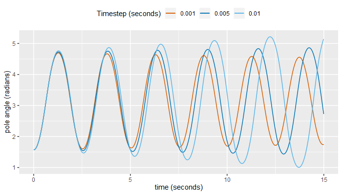
Figure 2 shows pole angle plots for three simulations based on Euler's method, with three different timestep durations of 1/1000th, 1/200th and 1/100th of a second, respectively. Note that the three simulations deviate significantly from each other within the 15 second simulation. Furthermore, in the two simulations with the largest timestep size (and thus largest approximation error) the pole is very clearly swinging to a higher maximum angle on each swing up, i.e. the pole is gaining energy on each swing in defiance of the law of conservation of energy, despite the presence of friction and the absence of any external forces adding energy to the system. This is a highly undesirable characteristic for a physical model that we may wish to simulate for longer than just a few seconds, as it makes the model in no way representative of the real world system it is attempting to simulate.

We now perform another set of three experiments, this time using the more accurate fourth-order Runge-Kutta method (RK4). For the three timestep sizes used in Figure 2, the three RK4 plots trace each other more or less exactly (not shown), i.e. there is no significant deviation between the three simulations. This is a strong indication that these plots are each tracing a path that is faithful to an equivalent real world experiment.

The logic here is that for the Runge-Kutta methods (and numerical methods generally) the approximation error decreases with decreases in timestep size, therefore if we observe a large reduction in timestep size not significantly reducing error, this implies the amount of error was negligible to begin with, i.e. there is no error (or only minimal error) in the simulations with the higher timestep size.

Figure 3 compares Euler's method and RK4 for the 1/1000th of a second timestep size:

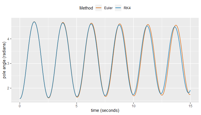
Figure 3 shows that Euler's method deviates from the RK4 path by a modest but significant amount even at a timestep size of 1/1000th of second, noting that we established above that the RK4 plot follows the correct path at the more coarse timestep size of 1/100th of a second. Note also that the maximum pole angle on each swing up is lower on each successive oscillation (both methods), as we would expect for a freely swinging pendulum with friction and no external force to maintain its motion.

We might now ask what the timestep size threshold is at which RK4 begins to deviate significantly from the correct path (in our limited experimental model that runs for just 15 seconds). Furthermore, we might ask what that threshold is for Euler's method, and for good measure we also include the standard form of the second-order Runge-Kutta method (RK2):

Table 5: Approximate maximum timestep size per method that results in an absolute pole angle error (at a simulation time of 15 seconds) less than 0.01 radians (approx. 0.57°)

Method	timestep (seconds)	Pole angle error at 15 seconds (radians, to 5 d.p.)
RK4	0.16(6) (1/6th)	-0.00836c
RK2	0.04 (1/25th)	0.00669c
Euler	0.0001 (1/10,000th)	0.00840c

Euler's method requires a timestep size in the order of 1000 times smaller than either RK2 or RK4 to ensure the approximation error remains below our chosen level. Therefore we do not recommend Euler's method if any degree of accuracy or faithfulness to an equivalent real world cart-pole system is required, especially over timescales longer than a few seconds. As such, the recommendation given here is to prefer RK2 or RK4 over Euler's method, and to choose a timestep size similar to those given in table 5.

6.3 General Procedure for Numerical Integration

The general procedure for applying the equations of motion in a simulation of the cart-pole system, is as follows:

1. Update the cart position $x$ based on the current cart velocity $\dot x$.


2. Update the pole angle $\theta$ based on the current pole angular velocity $\dot\theta$. Repeat for each pole in the multiple pole scenario.


3. Evaluate $\ddot x$ (based on the current state/positions, not the updated state).


4. Evaluate $\ddot\theta$, substituting in the calculated value for $\ddot x$ (again, based on the current state, not the updated state). Repeat for each pole in the multiple pole scenario.


5. Update the cart velocity $\dot x$ based on the current cart acceleration $\ddot x$, ready for use in the next timestep.


6. Update the pole velocity $\dot\theta$ based on the current pole angular acceleration $\ddot\theta$, ready for use in the next timestep. Repeat for each pole in the multiple pole scenario.

This procedure is essentially Euler's method applied to the cart-pole model state variables. Implementing a simulation using this procedure stands as a good first step towards implementing and understanding the higher order Runge-Kutta methods. A detailed description of those methods is outside the scope of this paper, but the high level procedure is essentially the same, with the difference being that the incremental changes applied to the state variables (the positions and velocities) are calculated by application of an iterative algorithm, whereas Euler's method applies a simple linear projection of the gradients. More details can be obtained by examination of the accompanying source code repository for this paper [6]:

6.4 Floating-point Precision Considerations

The simulations for obtaining the data for figures 2 and 3 utilised double-precision floating-point arithmetic and state variables. A repeat of those simulations based on single precision floating-point arithmetic showed no significant deviation in state from the double-precision simulations, with the RK2 and RK4 simulations being particularly robust when running in the lower precision mode. I.e. the errors inherent in Euler's method may be moderately exacerbated by the use of lower precision arithmetic, whereas the stability of the higher order RK2 and RK4 methods lends those methods to use of single precision arithmetic with no notable degradation in simulation fidelity.

7. Conclusions

We have presented step by step derivations for the equations of motion for the cart-pole system, with detailed supporting discussions. The below appendices provide further analysis and discussion of the equations appearing in the literature, and how they relate to the equations derived here. We hope that these in-depth derivations, analyses and discussions will provide a firm foundation for future research that utilises the cart and pole task in some capacity.

Appendix A: d'Alembert's Principle and Dynamic Equilibrium

As per Cannon [2] (§2.2, p.40) we adopt d'Alembert's view of dynamic equilibrium, whereby, for a system of rigid bodies, Newton's Second Law is written:

Where the $-ma$ term is considered to represent an inertial force that acts in the opposite direction to the external force F, and with equal magnitude. The inertial force is typically denoted with an asterisk, like so:

Giving:

Or more generally:

Where $f*$ represents all forces, external and inertial. I.e. for a system that is considered to be in a state of dynamic equilibrium, the sum of all external and inertial forces equals zero. This applies to the cart-pole compound body, and also to the cart and pole individually, considered in isolation from each other.

The same approach is adopted for rotational forces (moments, or torques), which can also be categorised as external and inertial forces. Where an inertial moment is a rotating mass' resistance to a change in the angular velocity.

Appendix B: Torque, or the Moment of Force

Torque is the rotational equivalent of force (or more specifically, the rotational equivalent of translational force).

If a force F is applied to the pendulum in figure 1 somewhere along its length, then the component of that force that is perpendicular to the pendulum rod (i.e. tangential to the current direction of rotation) will result in a rotational force on the pendulum; that rotational force is known as torque, or the moment of force. All other components of F that are not in the direction of rotation have no effect on its rotation.

The torque (moment) resulting from force F is given by the product of the aforementioned tangential component of F, and the distance from the rotational pivot point at which F is applied. E.g. a doubling of the distance from the pivot point at which F is applied results in a doubling of the resulting torque.

Torque is typically calculated by application of the cross product between a force vector (F) and a 'radial' vector projecting out from the pivot point to the point where force F is applied. The result is a vector parallel to the axis of rotation (i.e. perpendicular to the plane of rotation), the magnitude of which gives the torque's magnitude, and the direction of which gives the torque's direction (clockwise or anticlockwise).

By convention a positive torque describes an anticlockwise force (moment), and thus negative torque a clockwise moment; this convention is encompassed by the right hand rule, sometimes referred to as the right-handed screw rule; where a right-handed screw is one that advances into the material being screwed into when it is turned clockwise.

In our model (shown in figure 1) the axis of rotation is parallel to the z-axis, i.e. coming out of the page/screen, noting that the the convention for the z-axis is for a point coming out of the page to have a positive z coordinate, and a point going into the page to have negative z coordinate. Therefore, a right handed screw being turned clockwise into the page has a negative torque. This is somewhat inconsistent with our chosen scheme of the pendulum angle and angular velocity being positive in the clockwise direction, therefore some care needs to be taken with the signs of the torque equation terms.

Summarising; the moment of force, or torque $\boldsymbol{\tau}$, that results from a force $\mathbf{F}$ applied at position $\mathbf{r}$ relative to the centre of rotation, is given by the formula:

Where $\mathbf{F}$ and $\mathbf{r}$ are vectors, and $\times$ is the cross product. The result ($\boldsymbol{\tau}$) of this formula is a vector that projects along the rotation axis (i.e. in our model the vector projects out of, or into, the page at point P), and with a magnitude that represents the torque force (which is the quantity we are interested in, since we know the orientation of the fixed rotation axis).

There follows a short introduction to the concept of torque to provide some intuition and explanation of how the rotational force terms are derived.

Consider our pendulum rod with the mass removed and pivoted halfway along its length. The Law of the lever tells us how much a force $F_a$ applied on one side of the pivot point (at point $A$) translates to a force $F_b$ on the other side (at point $B$), given the distances $a, b$ of the two force points from the pivot:

I.e. $F_b$ varies linearly with the distance of $F_a$ from the pivot point. This is because for a given circular displacement of $A$, the resulting circular displacement of $B$ diminishes as $a$ increases. Those circular displacements are given by $ r\theta$, i.e. for an angular change of 360° ($= 2\pi^c$) the displacement becomes the circumference of a circle given its radius ($2\pi r$). Thus we can write the circular displacements $D_a, D_b$ in terms of $a, b$ and an angular change $\theta$:

We now express distance $b$ as a constant proportion of distance $a$:

I.e. the circular displacements of $A$ and $B$ are linearly proportional, and with the same linear factor as the relative distances of $A$ and $B$ from the pivot point.

Now consider change of circular displacement over time, taking the second derivative to give the circular acceleration of $A$ and $B$:

Once again expressing distance $b$ as a constant proportion of distance $a$:

Newton's Second Law ($F=ma$) tells us that force is proportional to acceleration, therefore a force $F_a$ applied at point A and perpendicular to the rod, will result in force $F_b = F_a / k$ at point B.

Appendix C: The Equations of Cannon

As noted above in section 3.4 and 3.5, equations (12) and (18) match the two equations of (22.55) in Cannon [2]. However, Cannon gives the following definition for the moment of inertia:

This is the moment of inertia for a pole with uniformly distributed mass, whereas all other aspects of Cannon's equations are based on a pendulum with a point mass at distance $l$ from the pivot point. This hybrid approach of combining equations for point and uniform mass is a deliberate choice, as it results in a set of equations that approximate the dynamics of the system reasonably well, without the additional complexity of the exact rotational force equations for a pole with uniform mass.

Cannon discusses in the book the importance of such simplifying approximations in the practical analysis of dynamic systems. A real world cart and pole system will be subject to many additional tiny forces that would be impractical if not impossible to accurately model in their entirety, such as forces caused by the rotation of the earth, the pull of gravity from the sun and moon, electro-magnetic forces caused by metal components interacting with the Earth's magnetic field, etc. Thus, the idealised cart and pole model is already a simplification of any real world system, and the choice to model the pole's rotational forces with a point mass results in equations that are broadly representative of the true dynamics, even if they are not exact.

However, there is a problem with Cannon's choice of definition for $J$ which goes beyond the choice to employ modelling approximations. Cannon derived equations based on a point mass halfway along the pole, representing the centre of mass of a pole with uniformly distributed mass; as such Cannon defined $l$ as the half length of the pole rather than full length as in the equations derived in this paper. The equations in [2] §22.55 match equations (12) and (18) above because both sets of equations are modelling a point mass at distance $l$ from the pivot point. The difference in the definition of $l$ manifests only in the choice of equation for $J$.

To properly apply equation (C1) to Cannon's model we must use the full length of the pole in that model, i.e. the rotational inertia for a pole with length $2\hat{l}$ is given by (where $\hat{l}$ represents the half length of the pole):

I.e. Using the half length $\hat l$ requires that $k=\frac{4}{3}$ is used, rather than $k=\frac{1}{3}$ as given by Cannon, and subsequently adopted elsewhere [1,5] (as discussed in appendices D and E).

As such, substituting $k=\frac{4}{3}$ into (26), (27) and (28) gives the following correct equations of Cannon:

From (26):

From (27):

From (28):

Noting the presence of $\frac{7}{3}$ factors rather than $\frac{4}{3}$. The $\hat{l}$ symbol acts as a reminder to use the pole's half length in these equations, and that these equations are intended to approximately model a pole with uniformly distributed mass, rather than exactly model a pendulum with a point mass.

Cannon [2] also contains two sign errors in the cross product terms that give the torque resulting from the inertial force caused by the inertial resistance of point mass Q. These errors are discussed in the notes box in section 3.5, but we shall discuss them further here. Fortunately these errors cancel each other out in the final equations, but they may result in some confusion for anyone wishing to follow the derivations given by Cannon.

The problem equations in Cannon are:

The corrected forms of these equations are:

I.e. in (22.53) the cross product term should not be prefixed with a minus sign; the resulting moment/torque from the cross product should be summed with the other moments to form the equilibrium equation. Noting that the last term has a minus sign only because the full definition for that term has been substituted in already, and that full term happens to have a minus sign (i.e. e.g. gravity pulling down on the pendulum at 90° results in a clockwise torque, and a clockwise torque has a negative sign).

Also note the minor typographic anomaly of $(\mathbf{1}_Rl)$ instead of $\mathbf{1}_R(l)$, which is the form used elsewhere in the book, and indeed in equation (22.54) which we discuss next.

The left hand side of equation (22.54) is prefixed with a minus sign. However, the right hand side is equivalent to the cross product without applying that minus sign. We believe that the cross product on the left hand side should not contain a minus sign, and thus the right hand side result is correct despite the left hand side error. Therefore when the right hand side is substituted into (22.53) the two sign errors cancel, giving the correct equations of motion given in (22.55).

Appendix D: The Equations of Barto et al.

Barto et al. [1] give the following equations of motion for a cart with a single pole, incorporating cart-track and cart-pole friction.

\begin{align} \ddot\theta &= \frac{g\sin\theta + \cos\theta \left[ \cfrac{-f -m\hat{l}\dot\theta^2\sin\theta + \mu_c\sgn(\dot x)}{m_c + m} \right] - \cfrac{\mu_p\dot\theta}{m\hat{l}}}{\hat{l} \left[ \cfrac{4}{3} - \cfrac{m\cos^2\theta}{m_c + m} \right]} \tag{D1} \\[6ex] \ddot x & = \frac{f + m\hat{l} \left[\dot\theta^2\sin\theta - \ddot\theta\cos\theta\right] - \mu_c\sgn(\dot x)}{m_c + m} \tag{D2} \\[6ex] g &= -9.8 \,m/s^2 \tag{D3} \end{align}

Symbols

$\tilde l$	Half length of the pole.
$m$	Mass of the pole.
$g$	Gravitational acceleration. -9.8 m/s2

Cannon [2] is cited as the origin of these equations, however, the cart-pole equations provided by Cannon do not include terms for friction forces. Cannon does discuss various models of friction (see [2] §2.2, pg42-43), and therefore it is likely that the cart-pole equations provided in [1] were extended using additional equations also from Cannon.

Equation (D1) can be rederived by rearranging equation (26-F) (with $l$ substituted with $\hat{l}$):

Equation (D2) is obtained with a minor rearrangement of (19-F) (again, with $l$ substituted with $\hat{l}$):

The rederived equations exhibit some discrepancies when compared to the equations given in [1], which we will now discuss.

Barto et al. [1] gives the wrong sign for $g$ in the table of symbols, i.e. equation (D1) is written in such a way that gravity is a downward force for a positive value of g. E.g. the $g\sin\theta$ term makes a positive contribution towards $\ddot\theta$ when the pole angle is between 0 and 180°, and g has a positive sign. Note also that in figure 1 of [1] $\theta$ is defined as the pole angle measured clockwise from the upright vertical, matching the scheme used in this paper, therefore the discrepancy with the sign of g hasn't come about through use of a different baseline/origin orientation for the pole.

It is not known if this gravity inversion was employed in the research performed in [1], or how many of the subsequent papers that adopted these equations also adopted the error (noting that at time of writing in November 2019, google scholar reports a citation count of 3,783). What can be said is that the cart-pole system was chosen as the subject of research because it is an unstable system, requiring an external dynamic controller to maintain stability. Whereas with inverted gravity the inverted pendulum becomes a normal pendulum, and is therefore no longer unstable. I.e. the system naturally settles into a state with the pole vertically up without an external controller.

Note that the $\frac{4}{3}$ term in (D1) is consistent with a value of $\frac{1}{3}$ for constant $k$ in equation (D4). Hence, equation (D1) has adopted the problematic moment of inertia term from Cannon [2], i.e. (D1) employs the moment of inertia for a pole of length $\hat{l}$, which is half of the pole's actual length (see appendix C for details).

The cart-track friction term of $\mu_c\sgn(\dot x)$ in (D1) and (D2) is consistent with equations (32) and (33), i.e. alternative simplified cart-track friction terms that do not take into account motion of the pole. This simplified friction force is in the opposite direction to the cart's movement (as expected), and is scaled by some constant, hence $\mu_c$ in [1] is essentially a combination of the co-efficient of friction and some other constant that represents a constant normal force. We prefer a cart-track friction term that is proportional to cart velocity [as per equation (34)] in order to avoid a discontinuity in the equations about zero velocity (see §3.8).

The cart-pole friction term in (D1) is proportional to the pendulum's angular velocity, and is therefore consistent with equation (40).

From Barto et al. [1]:

We initially used the Adams-Moulton predictor-corrector method to approximate numerically the solution of these equations, but the results reported in this article were produced using Euler's method with a time step of 0.02 s for the sake of computational speed. Comparisons of solutions generated by the Adams-Moulton methods and the less accurate Euler method did not reveal discrepancies that we deemed significant for the purposes of this article.

As per the discussion in section 6.2 and the results in table 5, it is likely that the experiments performed experienced some level of approximation error due to use of the simpler Euler method, but the authors did not consider the amount of error to be significant in the context of their experiments.

Appendix E: The Equations of Wieland

Wieland [5] gives the following equations of motion for the cart-pole model, incorporating cart-track and cart-pole friction. These equations are structured to allow for a cart with multiple poles attached, however here will consider a single pole only:

Symbols

$\tilde l$	Half length of the pole.
$\tilde F_i$	The effective horizontal force of the i'th pole on the cart.
$m$	Mass of the pole (for equations that relevant to a pole considered individually).
$m_i$	Mass of the i'th pole.
$\tilde m_i$	Effective mass of the i'th pole.
$\tilde\theta_i$	Angle of the i'th pole.
$g$	Gravitational acceleration. -9.8 m/s2

To obtain the equations for a single pole we substitute (E3) and (E4) into (E1), and rearrange:

Equation (E5) is compatible with (28-F), except for a difference in sign on the $mg\sin\theta\cos\theta$ term. Note however that Wieland [5] gives a negative value for g in table 1, therefore the two negatives cancel and thus (E5) is indeed compatible with (28-F).

Rearranging (E2) gives:

Equation (E6) is compatible with equation (27-F), noting once again that this form of the equation requires a negative value for g.

Note the $\frac{4}{3}$ terms in equations (E5) and (E6), these are consistent with a value of $\frac{1}{3}$ for constant $k$ in equations (27-F) and (28-F), hence the Wieland equations have adopted the problematic moment of inertia term from Cannon [2]. I.e. Wieland employs the moment of inertia for a pole of length $\hat{l}$, which is half of the pole's actual length (see Appendix C for details).

Equation (E5) gives a cart-track friction term compatible with equations (32) and (33) as per Barto et al. (see Appendix D for further discussion).

The cart-pole friction term in equations (E5) and (E6) is proportional to the pendulum's angular velocity, and is therefore consistent with equation (40) as per Barto et al. (see Appendix D for further discussion).

From Wieland [5]:

The single (unjointed) pole problems were modeled[sic] using the Euler method and a time step on[sic] 0.02 seconds. The multiple pole and jointed pole problems were modeled[sic] with a time step of 0.01 seconds and a fourth order Runge-Kutta model.

The numerical method applied for the single pole experiments mirrors the approach of Barto et al.[1], and therefore, as per the above discussion in section 6.2 and the results in table 5, it is likely that those experiments experienced some level of approximation error due to use of the simpler Euler method.

References

[1] Barto, Andrew G.; Sutton, Richard S. (1983) Neuronlike Adaptive Elements that can Solve Difficult Learning Problems. IEEE Transactions on Systems, Man, and Cybernetics, Vol. SMC-13 No.5, (1983) pp. 834-846     [link1]

[2] Cannon, Robert H. Dynamics of Physical Systems. New York: McGraw-Hill (1967)     [link1] [link2] [link3] [link4]

[3] Lunberg, Kent H.; Barton, Taylor W. (2009) History of Inverted-Pendulum Systems. IFAC Proceedings Volumes, Volume 42, Issue 24, 2010, pp. 131-135     [link1]

[4] Michie, D.; Chambers, R. A. (1968) BOXES: An Experiment in Adaptive Control.     [link1] [link2]

[5] Wieland, Alexis P. (1991) Evolving neural network controllers for unstable systems. Connectionist Models: Proceedings of the 1990 Summer School, ISBN 0-55860-156-2, pp. 91-102     [link1] [link2]

External Resources

[6] Accompanying source code: https://github.com/colgreen/cartpole-physics

Colin,
January 4th, 2020

Copyright 2020 Colin Green.
This article is licensed under a Creative Commons Attribution 3.0 License